Supervised learning: teaching algorithms to learn from example
Where we’ve been, where we’re going
In a previous post, we looked at neural networks from a high level - what they are, why they’re useful for biology, and how they fit into the broader machine learning landscape. We talked about perceptrons as computational units that learn to recognise patterns by adjusting weights.
Then we explored unsupervised learning - clustering methods that find structure in unlabelled data. K-means groups samples by similarity. Hierarchical clustering builds dendrograms showing nested relationships. Both are exploratory tools for when you don’t know what patterns exist.
Now let’s look at the other major branch: supervised learning. This is where you have labels. You know the answers. And you want an algorithm to learn the mapping from inputs to outputs so it can predict labels for new, unseen data.
This post unpacks the mathematics. How do these algorithms actually learn? What’s happening under the hood when we “train a model”? And what are the common failure modes to avoid?
The fundamental idea
Supervised learning means teaching an algorithm by example. You give your learning algorithm examples to learn from that include the correct answer or label (\(y\)) for every input feature (\(x\)), so that eventually you can just give an unlabelled input and the model will give a reasonably accurate prediction.
The more accurate this prediction, and the more unseen datasets you can apply the model to without sacrificing accuracy, the better the model overall.
- Model: A mathematical algorithm (often executed via a function or program), with variable parameters that have been optimised (the model has “learned” these values through training datasets) so that when applied to new input data, it can make reasonable output predictions
- x (features): These are the input variables or features used to make predictions. They represent the independent variables that influence the outcome
- y (target/labels): This is the variable we want to predict or classify. It represents the dependent variable (generally the last column of your dataframe)
- m: Often used as the standard symbol for the number of training examples in the dataset (rows/samples/observations)
- n: Similarly, n is used to denote the number of features (columns/variables/markers)
- \((x^{(i)}, y^{(i)})\): To refer to a single training example / sample / row of data
- \(x_j\): To refer to a single feature / trait / marker / column
- \(\hat{y}\): Referred to as “y-hat”, this represents a prediction of the output \(y\) based on the function or model \(f()\)
Two main types:
Regression: Predict a continuous numerical value. Gene expression levels in TPM. Growth rate in mm/day. Drought tolerance on a 0-100 scale.
Classification: Predict which category something belongs to. Disease-resistant or not. Cell type A, B, or C. High-risk or low-risk.
The better the predictions on unseen data, the better the model. Simple enough concept. Now let’s see how it actually works.
Starting simple: linear regression
The most intuitive place to start is with a straight line. Suppose you’ve measured expression for one gene across many grapevine samples, and you think this gene correlates with sugar content in the berries. Plot gene expression on the x-axis, sugar content on the y-axis, and you see a pattern - higher expression, higher sugar.
(This is an arbitrary example for illustration - nothing in biology is quite this simple, and gene expression rarely maps linearly to phenotype. But it gives us an intuitive starting point.)
A linear model takes the form:
\[f_{w,b}(x) = wx + b\]
Where: - \(w\) is the weight (the slope of the line) - \(b\) is the bias (the y-intercept) - \(x\) is your input feature (gene expression) - \(f_{w,b}(x)\) is the predicted output (sugar content)
This is univariate linear regression - one input feature. The goal is to find the values of \(w\) and \(b\) that make the line fit your data as closely as possible.
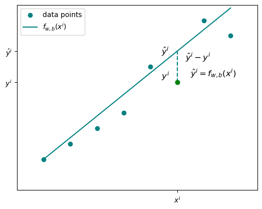
For any given sample \(i\), the predicted value is \(\hat{y}^{(i)} = f_{w,b}(x^{(i)})\). The actual measured value is \(y^{(i)}\). The difference between them is the error.
Measuring how wrong you are: the cost function
Once you’ve chosen values for \(w\) and \(b\), you need to know how well they work. Enter the cost function.
The error or loss for a single data point is:
\[L = \hat{y}^{(i)} - y^{(i)}\]
Or equivalently:
\[L = f_{w,b}(x^{(i)}) - y^{(i)}\]
But you don’t just care about one data point. You want a single value that represents how the model is performing over the entire dataset - all \(m\) samples. So we take the error for each example in the dataset and get a kind of average. This is exactly what the cost function does:
\[J(w, b) = \frac{1}{2m} \sum_{i=1}^{m} (f_{w,b}(x^{(i)}) - y^{(i)})^2\]
This is the mean squared error (MSE) cost function. A few things to note:
Why square the error? Two reasons. First, it removes negative values - errors above and below the line don’t cancel out. Second, it penalises larger errors more heavily. If you’re off by 10 instead of 1, the squared error is 100 times worse, not 10 times worse.
Why divide by \(2m\) instead of \(m\)? The \(1/m\) gives you the mean. The extra factor of \(1/2\) doesn’t change the optimisation (it’s just a constant), but it simplifies the derivative later when we do gradient descent. It’s a mathematical convenience.
The goal is clear: minimise \(J(w,b)\). Find the parameters where the cost is as small as possible.
Finding the minimum: gradient descent
So how do you find the minimum of the cost function? You could try plotting \(J(w,b)\) for every possible combination of \(w\) and \(b\), but that’s computationally ridiculous for anything beyond toy examples.
Instead, we use gradient descent.
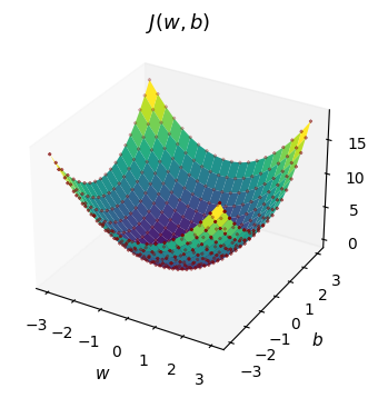
Imagine you’re standing on this surface somewhere random. You want to get to the lowest point. Gradient descent is simple: look around, figure out which direction is steepest downhill, and take a step in that direction. Repeat until you reach the bottom.
In essence, starting from any randomly chosen position for \(w\) and \(b\), the algorithm takes incremental and iterative steps in whichever direction the gradient is steepest - it finds the way to get to the bottom of the slope (the minimum) as efficiently as possible.
Mathematically:
\[w = w - \alpha \frac{\partial J(w, b)}{\partial w}\]
\[b = b - \alpha \frac{\partial J(w, b)}{\partial b}\]
Where: - \(\frac{\partial J(w, b)}{\partial w}\) is the derivative of the cost function with respect to \(w\) - it tells you the steepness of the slope - \(\alpha\) is the learning rate - it controls how big each step is - You subtract because you want to move down the slope
The values for the parameters \(w\) and \(b\) are repeatedly and simultaneously updated until the minimum is found, also known as convergence. Convergence happens when the parameter values are no longer significantly changing.
The learning rate matters. Too small, and convergence is painfully slow. Too large, and you overshoot the minimum, bouncing around without ever settling.
For simple linear regression, the cost function is convex - it has a single, bowl-shaped minimum. Gradient descent is guaranteed to find it eventually (assuming a reasonable learning rate). For more complex models, the landscape has multiple local minima, and where you start affects where you end up.
Scaling up: multiple features
One gene is rarely the whole story. You usually have multiple features - expression levels for several genes, or multiple SNP markers, or a combination of genomic and environmental measurements.
The model extends naturally to multiple linear regression:
\[f_{\vec{w},b}(\vec{x}) = w_1 x_1 + w_2 x_2 + \dots + w_n x_n + b\]
Now \(\vec{x}\) is a vector of features, and \(\vec{w}\) is a vector of weights. You can also write this as the dot product:
\[f_{\vec{w},b}(\vec{x}) = \vec{w} \cdot \vec{x} + b\]
The cost function looks the same, just vectorised:
\[J(\vec{w}, b) = \frac{1}{2m} \sum_{i=1}^{m} (f_{\vec{w}, b}(\vec{x}^{(i)}) - y^{(i)})^2\]
And gradient descent updates each weight independently:
\[w_j = w_j - \alpha \frac{\partial}{\partial w_j} J(\vec{w}, b)\]
The logic is identical. More features means more weights to optimise, but the underlying principle - minimise the squared error by following the gradient - stays the same.
The model can also extend to higher-order polynomials. If the relationship isn’t a straight line, you might have terms like \(x^2\) or \(x^3\) or interactions between features. The cost function remains MSE, but the function \(f_{\vec{w},b}(\vec{x})\) can now represent some higher-order equation, and the derivatives of the cost function with respect to these parameters may be more complex.
Beyond straight lines: classification with logistic regression
Predicting continuous values is useful, but biology often deals with categories. Is this plant drought-resistant or not? Does this sample belong to population A or population B? Is this mutation pathogenic?
Many biological questions involve classification of some kind, and linear regression models are not suitable for solving classification tasks. Enter logistic regression - despite the name, it’s a classification algorithm.
The core problem: linear regression outputs any real number. But for binary classification, you want a probability between 0 and 1. The solution is the sigmoid function:
\[g(z) = \frac{1}{1 + e^{-z}}\]
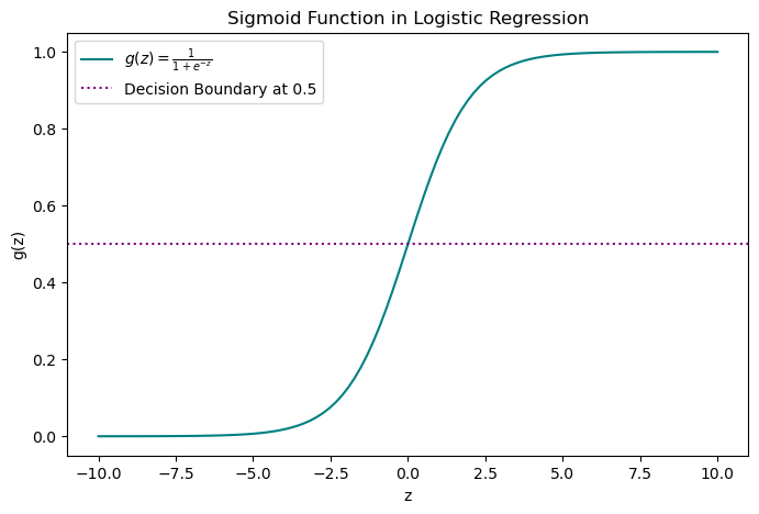
The sigmoid takes any input \(z\) and squashes it between 0 and 1. The tails approach 0 and 1 asymptotically but never quite reach them.
For logistic regression, \(z\) is your linear model:
\[z = \vec{w} \cdot \vec{x} + b\]
So the full prediction function becomes:
\[g(\vec{w} \cdot \vec{x} + b) = \frac{1}{1 + e^{-(\vec{w} \cdot \vec{x} + b)}}\]
The output is the probability that the sample belongs to the positive class. If the probability is above some threshold (typically 0.5), you classify it as positive. Below the threshold, negative.
The decision boundary is where the probability equals 0.5. If the decision boundary is linear (a straight line accurately divides the data into two categories), the value of \(z\) takes on the linear regression expression. However, if the decision boundary is best described by some other function or more complex polynomial, then \(z\) will change accordingly. In this way, the sigmoid function can accommodate complex data patterns with decision boundaries that are non-linear.
A different cost function for classification
Mean squared error doesn’t work well for logistic regression. The problem is that the sigmoid function makes the cost landscape non-convex - lots of local minima, and gradient descent gets stuck.
Instead, we use log loss (also called binary cross-entropy):
\[J(\vec{w}, b) = -\frac{1}{m} \sum_{i=1}^{m} \left[ y^{(i)} \log(g(z^{(i)})) + (1 - y^{(i)}) \log(1 - g(z^{(i)})) \right]\]
This looks intimidating, but the logic is straightforward:
- If \(y = 1\) (true label is positive), the cost simplifies to \(-\log(g(z))\)
- If \(y = 0\) (true label is negative), the cost simplifies to \(-\log(1 - g(z))\)
The effect: if the model predicts high probability for the correct class, the loss is small. If it predicts high probability for the wrong class, the loss is large. The model is penalised more when it’s confidently wrong.
Log loss is convex for logistic regression, so gradient descent works reliably.
The two ditches: overfitting and bias
As models get more complex - more features, higher-order polynomials, more parameters - two failure modes emerge.
Overfitting happens when the model fits the training data too precisely. It captures not just the underlying pattern but also the noise and random fluctuations. Training accuracy looks great. But the model doesn’t generalise - performance on new data is poor. Overfit models have high variance due to their sensitivity to noise.
Bias (or underfitting) is the opposite. The model is too simple to capture the real pattern. It misses the signal entirely. Both training and test accuracy are mediocre. Another way to think of bias is in the English sense of the word - a strong preconception that prevents the model from predicting the true values.
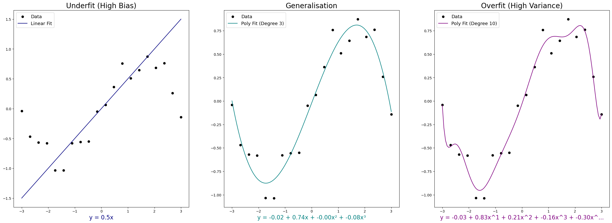
A model that generalises well avoids both extremes. It captures the underlying pattern without being distracted by noise.
How do you avoid these ditches?
Feature selection
If you have many features but few training samples, overfitting is likely. The model has too much freedom and not enough constraints. Overfitting can occur when there are many features in a model, but insufficient training examples. This could be solved by either collecting more data or, alternatively, by selecting a subset of features.
Feature selection involves choosing the most relevant variables in a dataset, which can significantly improve model accuracy while reducing computational costs and training time. Irrelevant features do not correlate with target labels and can add noise, increasing model complexity without improving predictive performance. Redundancy, or multicollinearity, occurs when multiple features that are correlated with the target labels are also highly correlated with each other, which can lead to overfitting.
Identifying the most relevant features in high-dimensional datasets is often challenging. In some cases, domain expertise can help guide feature selection, particularly when the dataset is small or well understood. However, if little is known about the biology of the features or if the dataset is high-dimensional, then reduction techniques such as PCA can be useful tools to inform these selections.
Ensemble methods like random forests or boosting combine multiple models trained on different subsets of features, reducing overfitting by averaging predictions.
Feature scaling or transformation - normalising features to a common range or standardising them (mean 0, standard deviation 1) - often improves model performance, especially for algorithms sensitive to feature magnitude.
Regularisation
Sometimes removing features entirely is too drastic. Regularisation offers a gentler approach - it penalises large weights instead of eliminating them.
The regularised cost function adds a penalty term:
\[J_{\text{reg}}(\vec{w}, b) = \frac{1}{2m} \sum_{i=1}^{m} (f_{\vec{w}, b}(\vec{x}^{(i)}) - y^{(i)})^2 + \frac{\lambda}{2m} \sum_{j=1}^{n} w_j^2\]
The new term \(\frac{\lambda}{2m} \sum_{j=1}^{n} w_j^2\) penalises large weights. The hyperparameter \(\lambda\) controls the strength of the penalty.
- If \(\lambda\) is too large, the model over-smooths and introduces bias
- If \(\lambda\) is too small (close to 0), regularisation has no effect
Tuning the value of \(\lambda\) is an important hyperparameter optimisation step to balance model complexity and generalisation.
This is L2 regularisation (or Ridge regression). The penalty is the sum of squared weights.
L1 regularisation (or Lasso) uses the absolute value of weights instead: \(\sum |w_j|\). This can shrink some weights all the way to zero, effectively performing feature selection.
Elastic net combines L1 and L2 penalties.
Regularisation works best when features are scaled, so the penalty isn’t skewed by large ranges.
Tying it back to neural networks
Remember the neural networks post where we talked about perceptrons? Each perceptron calculates a weighted sum of inputs, applies a threshold, and passes the signal forward if the threshold is exceeded.
That weighted sum? It’s \(\vec{w} \cdot \vec{x} + b\) - exactly the linear model we’ve been discussing.
The training process? Gradient descent minimising a cost function - exactly what we’ve just unpacked.
The difference is scale. A neural network is a collection of these units arranged in layers, with non-linear activation functions allowing the network to learn complex patterns. But the underlying mathematics - the cost function, the gradient descent, the weight updates - are the same principles we’ve covered here.
Deep learning isn’t magic. It’s supervised learning with many layers. The maths scales, but the logic remains.
The workflow in brief
Here’s what supervised learning looks like in practice:
- Collect and preprocess data - quality control, handle missing values, format correctly
- Feature engineering - select relevant features, transform or encode them appropriately (e.g., one-hot encoding for DNA sequences where A = [1,0,0,0], T = [0,1,0,0], etc.)
- Split the dataset - typically 60-70% training, 20-30% test, optionally 10-20% validation for hyperparameter tuning
- Train the model - optimise parameters by minimising the cost function via gradient descent
- Evaluate performance - check training error and test error to assess overfitting, bias, or generalisation
- Refine and iterate - tune hyperparameters, adjust features, try regularisation
Evaluating model performance with metrics
Model performance evaluation is performed with error analysis - comparing the fraction of the training and test datasets that the model has misclassified after training. If the model has high variance and is overfitting, the training error may be minimal, while the test error remains high. If there is bias, then both error values are likely to be high. When both error values are low, or as low as possible, then the model is generalising well and can be applied to unseen datasets. This “low-enough” error value can be decided on by setting a baseline level or benchmark for model performance, by looking to experimental studies, previous models generated on similar datasets, or an industry standard.
Besides error analysis, several metrics are commonly used to evaluate classification model performance:
Precision and recall: Precision refers to the accuracy of positive predictions - what proportion of positive predictions are true positives? (calculated as: true positives / (true positives + false positives)). Recall measures the sensitivity to positive predictions - what proportion of actual positives did we correctly identify? (calculated as: true positives / (true positives + false negatives)).
F1 score: This metric combines both precision and recall into one value using the harmonic mean: \(F1 = 2 \times \frac{P \times R}{P + R}\). Ideally, we want to balance high precision (high confidence in a positive prediction) with high recall (not missing too many true positives), since an inverse relationship often exists between them. When F1 is close to 1, there is balance between these values, but when it is close to 0, one of these metrics is too low.
AUROC: For imbalanced class distributions (where you have more data for some categories than others), the AUROC (area under the receiver operating characteristic curve) measure may be useful. This technique plots true positive rate against false positive rate at varying classification thresholds. The area under this curve can be interpreted as model performance, ranging from 0 to 1, with values closer to 1 indicating better performance.
Cross-validation: To further improve a model, the validation dataset is useful. Firstly, testing the data on different splits, instead of a single training/test split, gives a more robust measure of performance. After initial training, the validation set can be used to iteratively check the model performance, and to rotate the training and validation sets as many times as required to tune the hyperparameters in a process called cross-validation.
For now, the key takeaway: supervised learning is about finding a function that maps inputs to outputs by minimising a cost function. Gradient descent is the workhorse algorithm that does the optimisation. The challenge is balancing complexity (capture the pattern) with simplicity (don’t overfit the noise).
And those same principles underpin everything from linear regression to deep neural networks.
Further reading
- 3Blue1Brown’s gradient descent visualisation - exceptional visual explanations
- An Introduction to Statistical Learning - comprehensive, accessible textbook
- Deep Learning with Python (3rd edition) by François Chollet - excellent practical guide
- Andrew Ng’s Deep Learning Specialisation on Coursera - this course was a major inspiration for this post and provided the foundational understanding for many of these concepts. I think this is still a “gold standard” course if you want to dig deerer into these concepts.