Unsupervised learning: finding patterns without labels
Finding Structure in Unlabelled Data
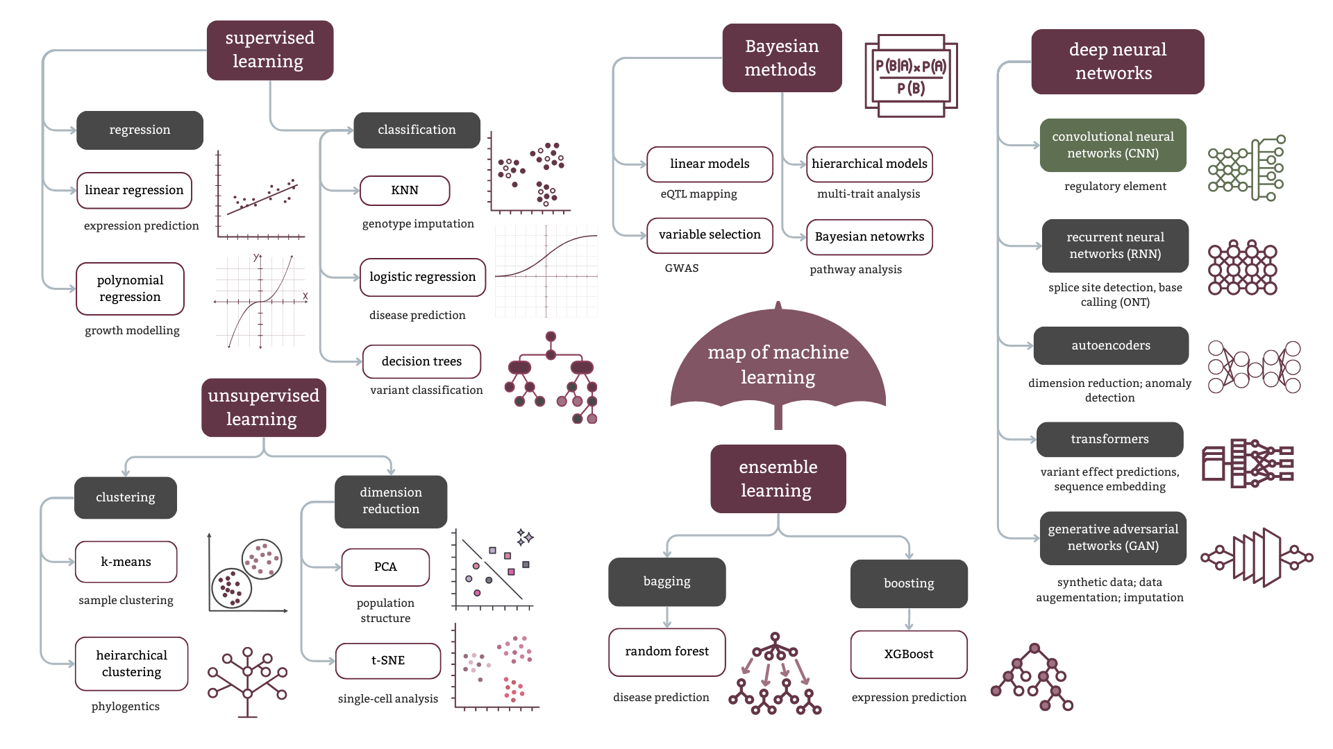
In this post’s plot, we explored the context “umbrella” of the machine learning landscape. Now let’s explore another major branch: unsupervised learning.
Unlike supervised learning - where you provide labelled input-output pairs for training - unsupervised learning identifies patterns in data without predefined categories. You’re not telling the algorithm what to look for; you’re asking it to find structure on its own. This makes it particularly useful during exploratory data analysis, when you don’t yet know what groups or patterns exist in your data.
The two primary approaches are clustering, which groups similar data points together, and dimensionality reduction, which simplifies high-dimensional data while preserving meaningful patterns. This post focuses on clustering. Dimensionality reduction with PCA has been covered in a separate post, here.
Clustering: Grouping the Similar
Clustering gives you a sense of the structure and distribution of a dataset. It identifies homogeneous groups based on distances between data points - samples that are “close” by some metric get grouped together. This is one of the most useful techniques during exploratory data analysis in genomics.
Let’s look at two foundational methods.
K-means Clustering
K-means is conceptually simple: you specify the number of clusters (\(K\)) you want, and the algorithm groups your data accordingly.
Here’s how it works. The algorithm calculates the Euclidean distance \(d\) between data points. For two points \(p\) and \(q\) with coordinates \((x_1, y_1)\) and \((x_2, y_2)\):
\[d(p, q) = \sqrt{(x_2 - x_1)^2 + (y_2 - y_1)^2}\]
Samples with minimal distance between them are assigned to the same cluster. Each cluster has a “centroid” - the centre point of all samples in that cluster. As new points are added, the centroid is recalculated iteratively by computing the mean position of all points in the cluster.
Choosing the Right K
How do you know how many clusters to use? One common approach is to calculate the sum of squared errors (SSE) for each cluster:
\[{SSE}_k = \sum_{i=1}^{n_k} (x_i - C_k)^2\]
where \(n_k\) is the number of points in the cluster, \(C_k\) is the cluster centroid, and \((x_i - C_k)^2\) is the squared Euclidean distance between each point and the centroid.
You sum the individual cluster SSE values to get a total SSE (\(SSE_T\)), then repeat this for different values of \(K\). Plotting \(SSE_T\) against \(K\) gives you an “elbow plot” - the \(SSE_T\) typically decreases as \(K\) increases, but at some point the rate of decrease slows down. That inflection point, the “elbow”, suggests the optimal number of clusters.

The method is somewhat subjective and often requires domain expertise to interpret correctly. Is the elbow at \(K\) = 3 or 4? It depends on your biological question.
Example: Gene Expression Under Stress
Here’s a simple illustration. Suppose you’ve measured expression levels for many genes under drought stress and normal conditions in wheat. Each data point represents a gene, and the axes represent expression levels under the two conditions.

With \(K\) = 4, you differentiate between genes that are highly expressed under drought but show varying expression under normal conditions. With \(K\) = 3, those groups are collapsed. Neither is “wrong” - the choice depends on what you’re trying to understand.
K-means has been effective for identifying clusters of co-expressed genes from microarray data, where each cluster might correspond to a specific phenotype like height ranges in wheat or cancer subtypes. The algorithm is straightforward and computationally efficient, but it’s sensitive to the initial placement of centroids and your choice of \(K\). Many implementations focus on improving the initialization step to achieve more stable convergence and better quality clusters.
If you don’t know the number of clusters in advance, or if you want to understand relationships between clusters, hierarchical clustering is a better option.
Hierarchical Clustering
Hierarchical clustering groups data points based on pairwise similarity, producing a tree-like structure called a dendrogram that reveals nested relationships between clusters.
It can be performed in two ways:
- Agglomerative (bottom-up): Each data point starts as its own cluster, and similar clusters merge iteratively until you have one big cluster.
- Divisive (top-down): All data points start in one cluster, which is recursively split into smaller clusters.
The structure of the dendrogram depends on two key choices: the distance measure and the linkage criterion.
Distance Measures
Euclidean distance (the formula above) is common for continuous variables, but it’s sensitive to differences in magnitude between features, so you typically need to normalize your data first. Manhattan distance - the sum of absolute differences between corresponding data points - can be more robust to large individual variations. Many specialized distance measures exist depending on the application, particularly for sequence data.
Linkage Criteria
Linkage determines how clusters merge:
- Single linkage: Uses the shortest distance between any two points in different clusters. This tends to form chain-like structures.
- Complete linkage: Uses the largest distance between points in different clusters. This produces more compact clusters.
- Average linkage: Averages distances between all pairs of points across clusters. This balances the extremes.
Your choice of distance measure and linkage criterion directly affects the dendrogram structure and, ultimately, the biological interpretation of your clusters.
Applications in Biology
Hierarchical clustering is widely used in gene expression studies, though it can lack robustness depending on the data. It also underpins many phylogenetic algorithms that infer evolutionary relationships from sequence data.
Phylogenetic clustering often uses sequence-specific distance measures like alignment scores or substitution models. Common methods include UPGMA (Unweighted Pair Group Method with Arithmetic Mean), Neighbour-Joining, Maximum Parsimony, Maximum Likelihood, and Bayesian inference approaches. The choice of distance metric, alignment method, and model assumptions significantly influences the inferred evolutionary relationships.
Beyond Clustering
Clustering is just one branch of unsupervised learning. The other major approach - dimensionality reduction - tackles a different problem: how do you visualize or analyze data with hundreds or thousands of features?
Techniques like Principal Component Analysis (PCA) and t-SNE help simplify high-dimensional datasets by transforming them into lower dimensions while preserving the most meaningful patterns. These methods are particularly useful for exploratory analysis of genomic data, where you might have expression measurements for 20,000 genes but need to understand the overall structure. I’ve put together a full PCA theory and practical tutorial in a seperate blog post.